VRAI

1. Teaching a student analogy

Training an AI model is surprisingly similar to how a human teacher helps a student master a new skill, like solving math problems:

Demonstration (Recorded Data): In robotics, the roboto needs a dataset, a list of examples of what to do : recorded human demonstrations. Think of a student who would ask the teacher for many examples of solved problems.
Practice (Prediction): The model takes into account the current state of the environment (vision, positions) and attempts to predict the correct actions to do. Similarly, a student may randomly pick a solved problem (from that list of solved problems) and try to solve it on their own.
Grading (Loss Function): The AI uses a loss function to mathematically measure the difference between its predicted actions and the actual actions demonstrated by the human teacher. A student will need the teacher to grade their work, showing them how far off they were from the correct answer.
Improvement (Optimization): The AI uses the loss to tune its parameters using an optimization algorithm, reducing its errors over time. The student will use the teacher's feedback (the loss) to correct their mistakes and improve for the next test.

To sum up, we need example, attempts, a feedback, and an optimizer. Let's see how it works in practice with a concrete example. For example, consider a robot that needs to pick up a block and place it on a target.

The Task

Below is an illustration of our task. After training, the robot should be able to pick up the block and place it in the target on its own, without human intervention.

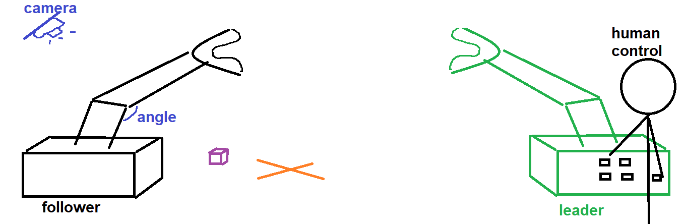
To get our examples, we use a leader-follower robot system where a human teleoperates the leader arm to demonstrate the task. The follower arm then uses the orders of the learder arm. Sensors and cameras record the data of the follower arm while it replicates the task. The dataset is then ready. Then, the ACT (Action Chunking Transformer) architecture lets the robot try to complete the task, grades the robot, and finally helps the robot improve its strategy over time. Let's dive into the training process and see how the algorithm works in detail.

2. The Training Phase: Breaking Down Algorithm 1

Below is a figure from the research paper Learning Fine-Grained Bimanual Manipulation with Low-Cost Hardware describing the steps of the training process.

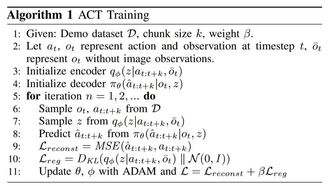
Here, we will break down the training phase described in the algorithm.

Step 1: The Initial Setup

The algorithm starts by defining three key components:

Dataset $\mathcal D$: The complete collection of our recorded human demonstrations.
Chunk Size ($k$): This defines how many consecutive actions the model will try to predict at once. Instead of predicting one single micro-movement at a time, it predicts a continuous "chunk" of movements.
Constant ($\beta$): A mathematical balancing factor (beta) that we will discuss later. For now, it doesn't matter much.

Step 2: The Examples ($o_t$ and $a_t$)

During the demonstration, we continuously record pairs of data: what the robot "sees and feels" and what it "does".

The Observation Data ($o_t$)

The robot has sensors that measure the precise angles of its various joints and motors. We can call it proprioception: it's the same sense that allows you to know your arm is raised even if your eyes are closed. Simultaneously, cameras record visual data of the environment. Using some math/AI tools (like Convolutional Networks and Multi-Layer Perceptrons), these visual and physical signals are compressed into long, very rich, and very informative vectors. Together, this combined physical and visual awareness creates the observation ($o_t$) at a specific time $t$.

The Action Data ($a_t$)

At that exact same time $t$, we record the action (the command) sent to the robot, for instance, "move the gripper 2cm to the left". In reality, this action is the physical movement of a "leader" arm controlled by a human experimenter. Just like the observations, this action information is translated into complex mathematical vectors that capture specific, subtle details about the movement, going far beyond a simple text description.

Steps 3 & 4: Initialization

Think of an AI model as a complex machine with millions of dials, cursors, and parameters. During training, these configurations are slowly optimized so the AI can perform its job perfectly. However, at the very beginning (Steps 3 and 4), the machine's architecture is built, but all those dials are set to random positions.

Imagine a person on their first day of work with no instruction manual, turning knobs at random and hoping for the best. Or, picture a student who skipped classes and hasn't studied at all showing up to a test! Their initial predictions are completely random and highly unlikely to be efficient or correct.

Steps 5 to 8: The Training Loop

Step 6 : Drawing data from the dataset

Now the actual learning starts. We pull a bunch of training examples from our dataset (a set of observations and the actual list of actions performed by the human experimenter). This is equivalent to a student selecting some of the practice problems with the teacher's complete worked-out solutions.

Step 7 : Extracting the "Style" variable, $z$

There are often multiple correct ways to complete a task. Imagine asking 1,000 people to brush their teeth. Everyone will do it slightly differently. Everyone has a "style." The AI uses the recorded actions and proprioception to extract a mathematical representation of this style (represented by the variable $z$). Returning to our analogy, this is like the student analyzing the answer keys and trying to figure out the teacher's specific problem-solving style (e.g., do they prefer long, rigorous calculations or clever theoretical shortcuts?).

Step 8 : Predicting the Actions

Armed with the current observations (the student now looking at the problem without the solution) and the extracted style (the student having an idea of the teacher's method in mind), the AI then tries to predict the precise sequence of actions required to complete the task (the student tries to write the solution of the problem based on what they understand so far).

Step 9: Grading the Actions (The Primary Loss)

Once the AI makes its predictions, we compare its predicted actions directly against the actual actions that were performed by the experimenter. We mathematically "grade" the model's prediction. This is exactly the same as a teacher taking out a red pen to grade the accuracy of a student's final answer. The bigger the mistake, the worse the grade (or "loss").

Step 10: Grading the Style (The KL Divergence)

This step is a bit harder to interpret at a high level, but it is crucial. Once deployed in the real world, the robot needs to operate reliably using a "standard" style. If the AI learns highly eccentric or chaotic styles during training, it might fail when acting on its own.

Think back to our brushing teeth analogy: there is a standard, generally accepted way to do it. In this step, we grade how "fancy" or "non-standard" the styles generated by the AI are. We are essentially telling the model: "Don't be too creative." It's like the teacher giving additional feedback to the student, not just grading if the final answer is right, but telling them: "Your solution works, but your solution is too chaotic. Please be more organized and stay closer to my method."

Step 11: Improving for the Next Test (Optimization)

After receiving their graded exam, a good student studies their mistakes to improve their understanding before the next test. The AI does exactly the same thing. It looks at its overall "grade" (the calculated loss) and uses an optimization algorithm (ADAM) to slightly adjust all of its internal dials and parameters. These adjustments ensure that its performance will be slightly better in the next round.

This entire cycle: "1) Pulling examples, 2) Making predictions, 3) Getting graded, and 4) Updating parameters" is repeated thousands of times until we are satisfied with the AI's training. Once training is complete, the robot is finally ready to act on its own in the real world. This next phase is called Inference.

3. The Inference Phase: the AI controls the robot

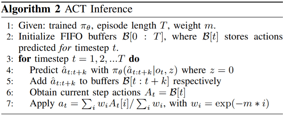
With the training phase complete, the robot is ready to perform tasks autonomously. Let's look at Algorithm 2, which outlines the steps of this inference phase.

Step 1 and 2: Initialization

After training the AI, we have a fully functional policy (denoted as $\pi_\theta$). This is essentially how the robot has learnt to complete the task it was taught. Ready to be used, this policy will continuously compute action chunks, which are sequences of actions the robot intends to perform.

As the robot generates these sequences, they need to be stored somewhere before they are executed. They are placed into a temporary holding area, or a queue, labeled $\mathcal B$. At the very beginning of the task, this queue is initialized and starts completely empty.

Step 3: The Inference Loop

The robot now enters a continuous loop, where it observes its surroundings, processes that information through its neural network, and executes actions until the task is complete.

Steps 4 & 5: Predicting the Action Chunk

As we saw during the training phase, the AI learned to associate actions with a specific "style" (the variable $z$). During inference, we want the robot to be reliable rather than creative, so we generate the action chunk using a standard, neutral style (mathematically represented as $z=0$).

By combining this standard style with its current observations (the live camera feeds and its physical state), the policy predicts a complete action chunk (denoted as $\hat a$). Indeed, instead of deciding what to do for just the next millisecond, the robot plans out a short sequence of $k$ future steps: $\hat a_{t:t+k}$. This is the step 4.

Step 5 is simply adding this entire planned sequence to our queue, $B$, which we initialized earlier.

Steps 6 & 7: Temporal Ensembling

Because the robot continuously predicts action chunks as it moves, these chunks naturally overlap. This means that for any specific moment, the robot actually has several different predicted actions to choose from.

How does it decide which one to follow? This is where Step 7 comes in. Instead of just picking one, the robot takes a weighted average of all overlapping predictions. Predictions made further in the past might be slightly obsolete because the environment has since changed. Therefore, the robot gives much higher weight to the most recent predictions, as they were calculated using the most up-to-date observations of its state and surroundings.

The Final Loop: Task Completion

This process 1) observing, 2) predicting chunks, and 3) averaging overlapping plans, repeats continuously. The robot persists in this cycle until it reaches the end of the episode and the specified action is successfully completed!

ACT: Action Chunking Transformer